NB! This tutorial is based on the Whitebox Workflows for Python (WbW) Tutorial 2: Geomorphometric Analysis
1. Download sample data
library(wbw)

# Download sample dataset
sample <-
  wbw_download_sample_data(
    data_set = "Grand_Junction",
    path = tempdir()
  )

# Load as WhiteboxRaster
dem <- wbw_read_raster(file.path(sample, "DEM.tif"))
dem
#> +---------------------------------------------+
#> | WhiteboxRaster                              |
#> | DEM.tif                                     |
#> |.............................................|
#> | bands       : 1                             |
#> | dimensions  : 1751, 1812  (nrow, ncol)      |
#> | resolution  : 5.000000, 5.000000  (x, y)    |
#> | EPSG        : 32612  (not specified)        |
#> | extent      : 749229 758284 4382303 4391053 |
#> | min value   : 1814.211060                   |
#> | max value   : 2599.727051                   |
#> +---------------------------------------------+
2. Fill missing data
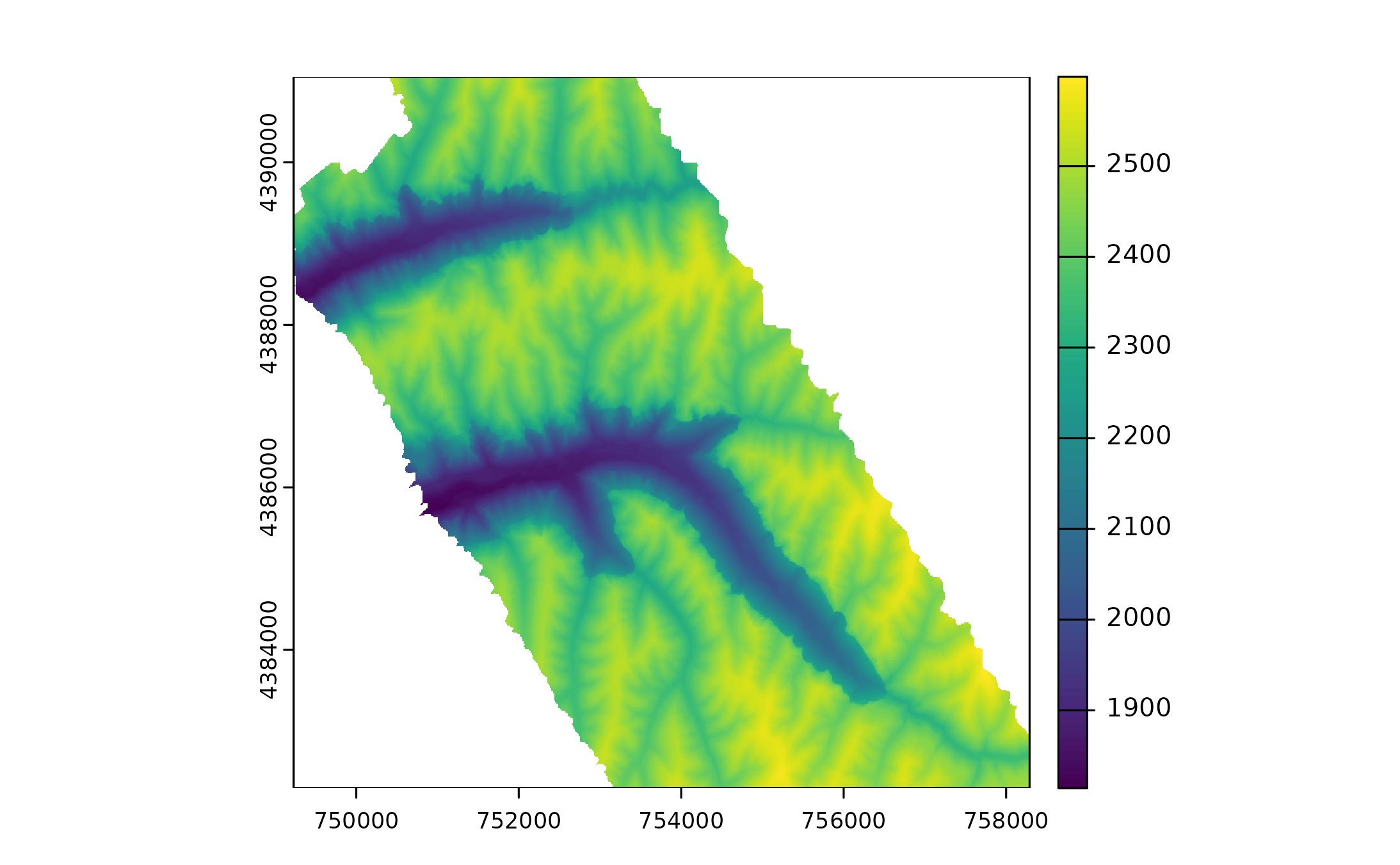
However, there are some missing values presented in the DEM.

To fill them, one can use wbw_fill_missing_data
function:
dem_filled <-
  wbw_fill_missing_data(dem, filter_size = 35, exclude_edge_nodata = TRUE)

dem_filled |>
  as_rast() |>
  plot()
3. Vizualization
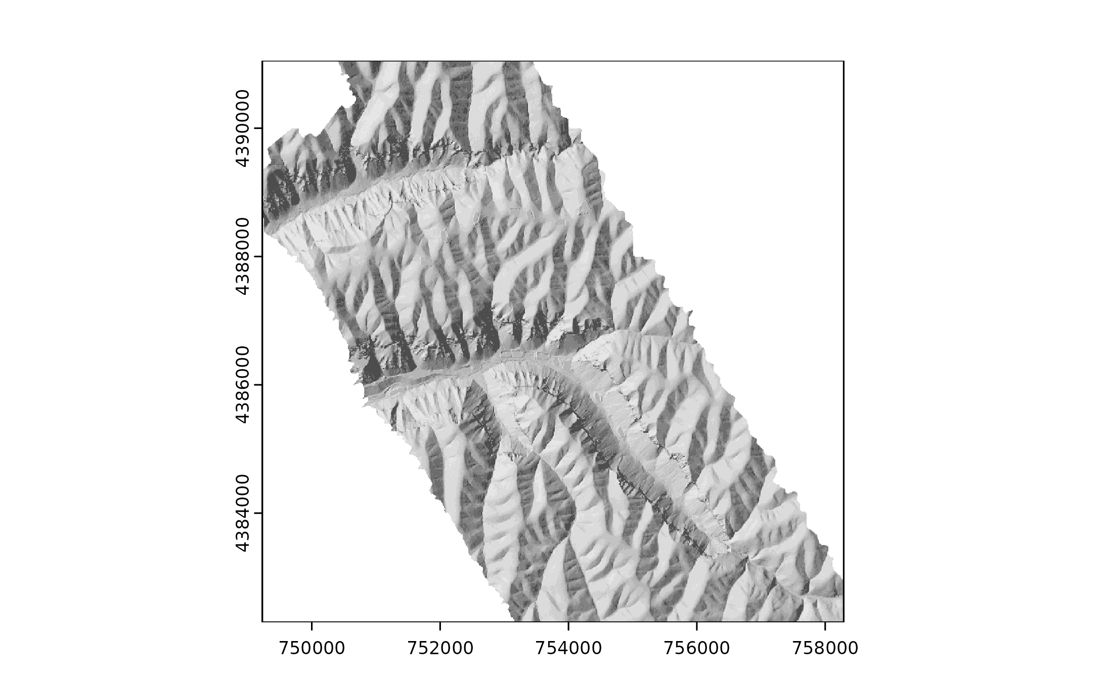
To properly vizualize the DEM, let’s create a hillshade map of the relief:
dem_hillshade <- wbw_multidirectional_hillshade(dem_filled)

dem_hillshade |>
  as_rast() |>
  plot(col = gray.colors(10), legend = FALSE)
4. Raster summary stats
One can get WhiteboxRaster summary statistics by running
familiar functions from base R (and terra):
# Raw DEM
wbw_cols(dem) # Number of columns
#> [1] 1812
wbw_rows(dem) # Number of rows
#> [1] 1751
num_cells(dem) # Number of cells
#> [1] 3172812
wbw_res(dem) # Raster resolution
#> [1] 5 5

# NA-Filled DEM
wbw_cols(dem_filled) # Number of columns
#> [1] 1812
wbw_rows(dem_filled) # Number of rows
#> [1] 1751
num_cells(dem_filled) # Number of cells
#> [1] 3172812
wbw_res(dem_filled) # Raster resolution
#> [1] 5 5

# Number of NoData values:
waldo::compare(
  sum(is.na(as_vector(dem))),
  sum(is.na(as_vector(dem_filled)))
)
#> `old`: 1361618
#> `new`: 1357688
5. Extracting land-surface parameters (LSPs)
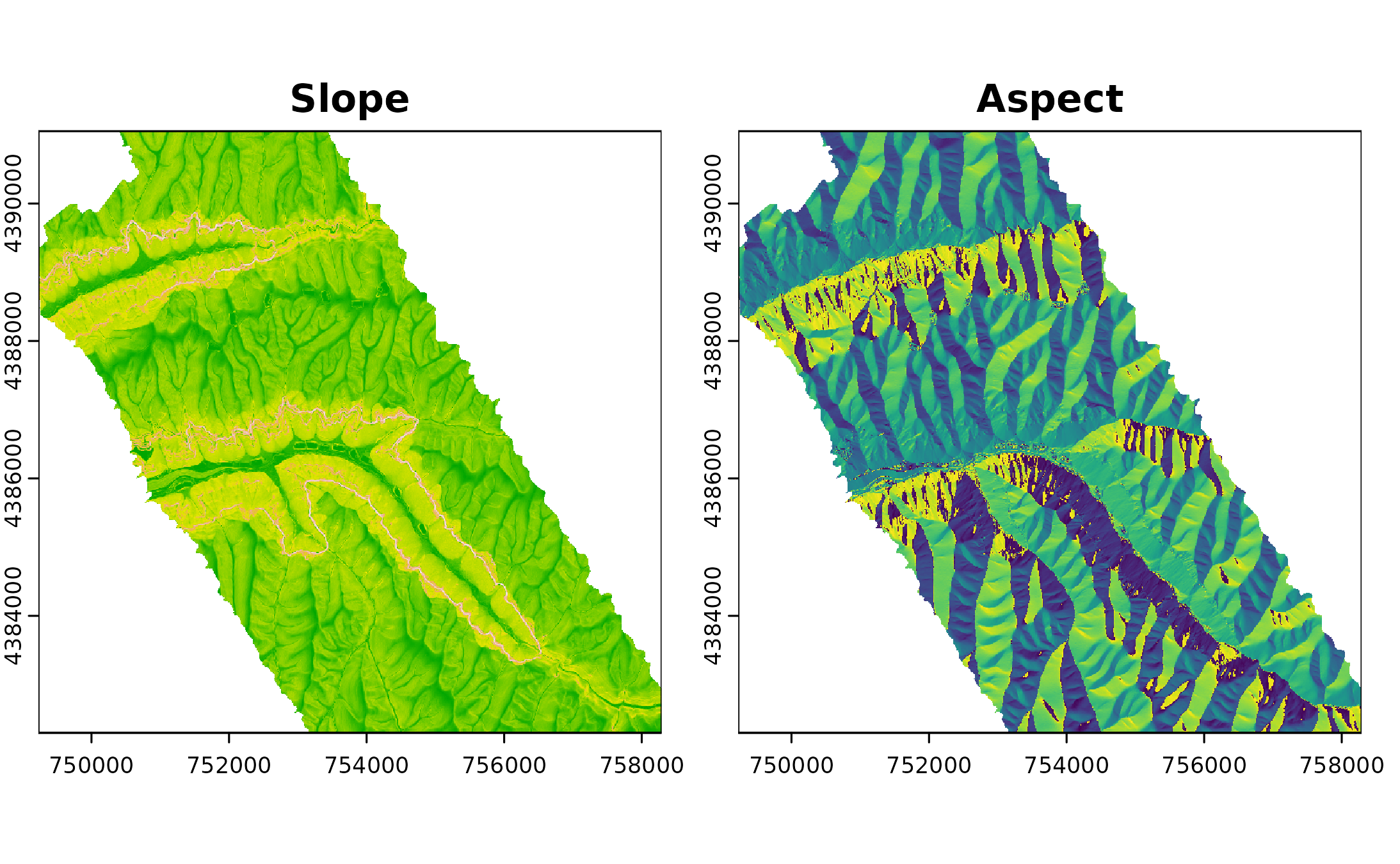
Now let’s extract some common land-surface parameters (LSPs), the basic building blocks of a geomorphometric analysis.
Slope and Aspect
# Slope
slope <- wbw_slope(dem_filled)
aspect <- wbw_aspect(dem_filled)

# Set up a 1x2 plotting layout
par(mfrow = c(1, 2))

# Plot the first raster (Slope)
plot(as_rast(slope),
     main = "Slope",
     legend = FALSE,
     col = terrain.colors(100),
     mar=c(1,1,1,1))

# Plot the second raster (Aspect)
plot(as_rast(aspect),
     main = "Aspect",
     legend = FALSE,
     mar=c(1,1,1,1))
