To evaluate the performance of different R packages for terrain analysis, here three different implementations are benchmarked:
- wbw (WhiteboxWorkflows for R): this package
- whitebox (WhiteboxTools for R): A traditional command-line based approach that writes results to disk
- terra: R’s leading package for raster processing, using an optimized C++ backend
Hillshade
The traditional hillshading, repeating the procedure from the
terra::shade() documentation. Each process was run 21
times.
# Load libraries
library(wbw)
library(whitebox)
library(terra)
# Load file
f <- system.file("extdata/dem.tif", package = "wbw")
# Create a tempfile for {whitebox}
tmp <- tempfile(fileext = ".tif")
bench_hillshade <-
bench::mark(
wbw = {
wbw_read_raster(f) |>
wbw_hillshade(
azimuth = 270,
altitude = 40
)
},
whitebox = {
whitebox::wbt_hillshade(
f,
azimuth = 270,
altitude = 40,
output = tmp,
compress_rasters = FALSE
)
},
terra = {
r <- terra::rast(f)
s <- terra::terrain(r, "slope", unit = "radians")
a <- terra::terrain(r, "aspect", unit = "radians")
terra::shade(
slope = s,
aspect = a,
angle = 40,
direction = 270,
normalize = TRUE)
},
check = FALSE,
time_unit = "ms",
iterations = 21L
)
bench_hillshade
#> # A tibble: 3 × 6
#> expression min median `itr/sec` mem_alloc `gc/sec`
#> <bch:expr> <dbl> <dbl> <dbl> <bch:byt> <dbl>
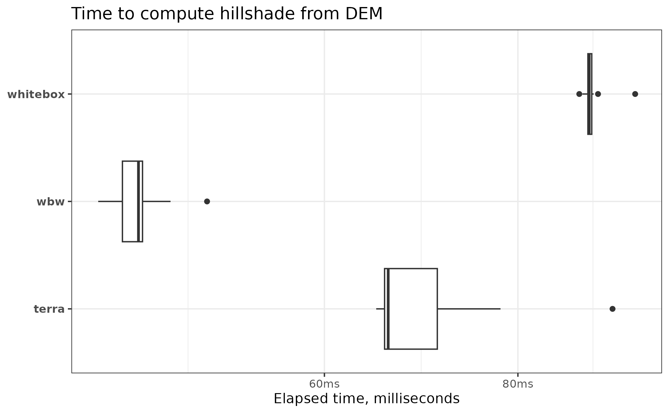
#> 1 wbw 44.2 45.4 21.9 681KB 0
#> 2 whitebox 88.4 89.8 11.1 94.9KB 0
#> 3 terra 64.5 67.1 14.4 103.2KB 0.720All three packages performed adequately, with wbw being
1.48 times faster than terra and 1.98 times faster than the
original whitebox. While with the latter, the raster object
is not yet loaded into the R session.
library(ggplot2)

ggplot2::autoplot(bench_hillshade, type = "boxplot") +
  ggplot2::labs(
    title = "Time to compute hillshade from DEM",
    y = "Elapsed time, milliseconds",
    x = NULL
  )
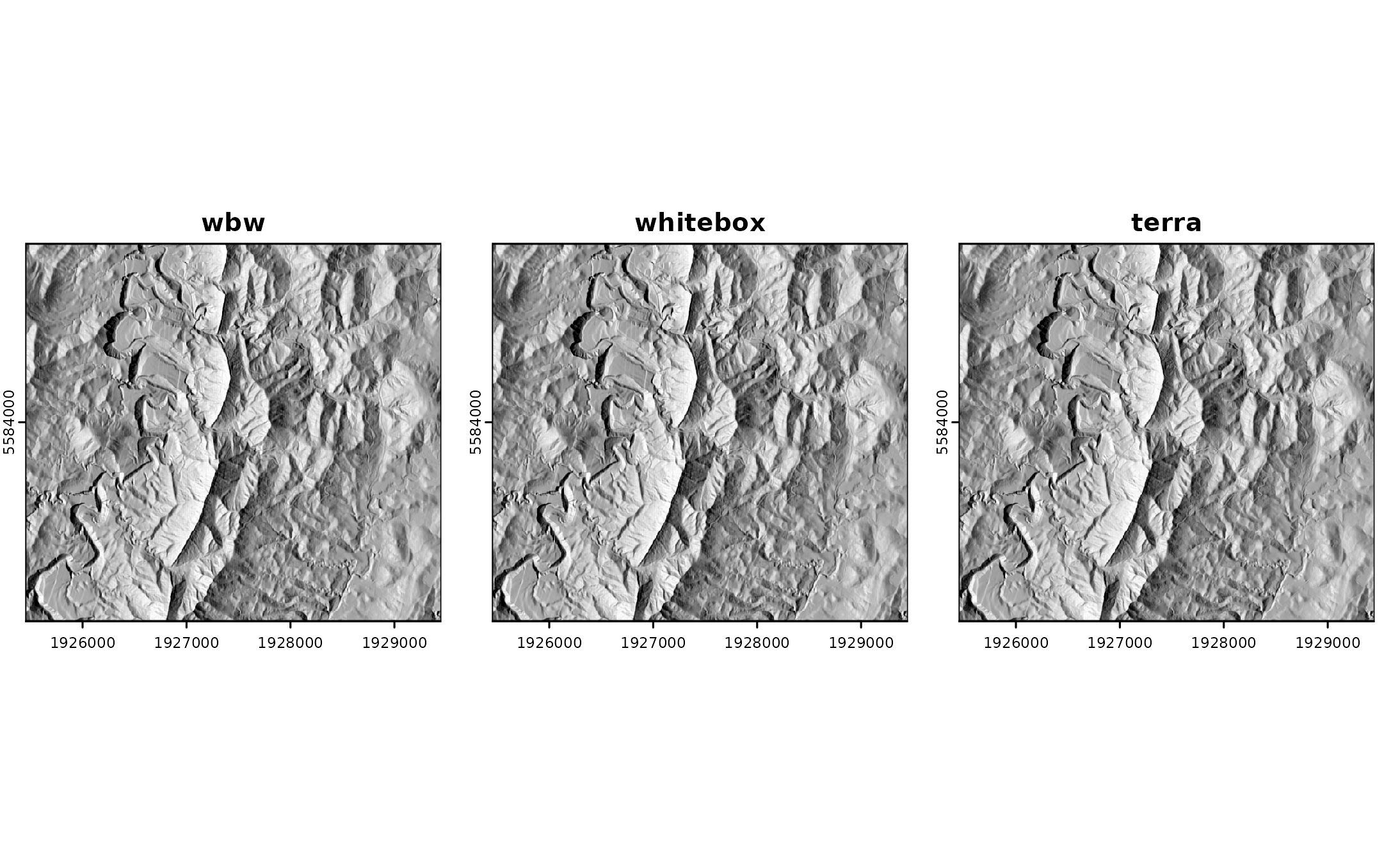
One can plot all hillshades next to each other to ensure that they all look alike.
# wbw
wbw_hillshade <-
  wbw_read_raster(f) |>
  wbw_hillshade(
    azimuth = 270,
    altitude = 40
  ) |>
  as_rast()

# whitebox
wbt_hillshade <- terra::rast(tmp)

# terra
r <- terra::rast(f)
s <- terra::terrain(r, "slope", unit = "radians")
a <- terra::terrain(r, "aspect", unit = "radians")
terra_hillshade <-
  terra::shade(
    slope = s,
    aspect = a,
    angle = 40,
    direction = 270,
    normalize = TRUE
  )

# Set up a 1x3 plotting layout
par(mfrow = c(1, 3))
clrs <- grey(0:100/100)

# wbw
plot(wbw_hillshade,
  main = "wbw",
  legend = FALSE,
  col = clrs,
  mar = c(1, 1, 1, 1)
)

# whitebox
plot(wbt_hillshade,
  main = "whitebox",
  legend = FALSE,
  col = clrs,
  mar = c(1, 1, 1, 1)
)

# terra
plot(terra_hillshade,
  main = "terra",
  legend = FALSE,
  col = clrs,
  mar = c(1, 1, 1, 1)
)
Terrain Parameters
When it comes to slope estimation, the difference between packages is not that significant.
# Create a tempfile for {whitebox}
tmp <- tempfile(fileext = ".tif")

bench_slope <-
  bench::mark(
    wbw = {
      wbw_read_raster(f) |>
        wbw_slope()
    },
    whitebox = {
      whitebox::wbt_slope(
        f,
        output = tmp,
        compress_rasters = FALSE
      )
    },
    terra = {
      terra::rast(f) |>
        terra::terrain("slope")
    },
    check = FALSE,
    time_unit = "ms",
    iterations = 21L
  )

bench_slope
#> # A tibble: 3 × 6
#>   expression   min median `itr/sec` mem_alloc `gc/sec`
#>   <bch:expr> <dbl>  <dbl>     <dbl> <bch:byt>    <dbl>
#> 1 wbw         41.2   42.4      23.4  125.32KB        0
#> 2 whitebox    82.5   83.9      11.8   25.23KB        0
#> 3 terra       23.2   24.3      41.0    6.75KB        0
Raster Summary Stats and I/O
As a rule of thumb, majority of in-memory operations happens
similarly fast in wbw compared to terra. Mind
the difference in performance for the slope estimation when rasters are
loaded into R session.
# Load libraries
library(wbw)
library(terra)

# Load file
f <- system.file("extdata/dem.tif", package = "wbw")
w <- wbw_read_raster(f)
r <- terra::rast(f)

# Conversion raster to matrix
bench::mark(
  wbw = as_matrix(w),
  terra = as.matrix(r, wide = TRUE),
  check = TRUE,
  time_unit = "ms",
  iterations = 21L
)
#> # A tibble: 2 × 6
#>   expression   min median `itr/sec` mem_alloc `gc/sec`
#>   <bch:expr> <dbl>  <dbl>     <dbl> <bch:byt>    <dbl>
#> 1 wbw        42.5   42.7       23.4    4.55MB     5.50
#> 2 terra       4.02   4.23     232.     8.87MB    72.6

# Estimating true mean
bench::mark(
  wbw = mean(w),
  terra = global(r, "mean")$mean,
  check = TRUE,
  time_unit = "ms",
  iterations = 21L
)
#> # A tibble: 2 × 6
#>   expression   min median `itr/sec` mem_alloc `gc/sec`
#>   <bch:expr> <dbl>  <dbl>     <dbl> <bch:byt>    <dbl>
#> 1 wbw         2.64   2.67      370.    2.83KB        0
#> 2 terra       4.62   4.73      168.   82.08KB        0


# Estimating slope
bench::mark(
  wbw = wbw_slope(w),
  terra = terrain(r, "slope"),
  check = FALSE,
  time_unit = "ms",
  iterations = 21L
)
#> # A tibble: 2 × 6
#>   expression   min median `itr/sec` mem_alloc `gc/sec`
#>   <bch:expr> <dbl>  <dbl>     <dbl> <bch:byt>    <dbl>
#> 1 wbw         35.8   36.5      27.2        0B        0
#> 2 terra       18.7   18.9      52.8    3.13KB        0
However, this happens because terra is not actually
loading the whole raster into memory, unlike wbw.
Therefore, the input operations are much faster for
terra, while the output operations are more
efficient in wbw.
# Reading raster
bench::mark(
  wbw = wbw_read_raster(f),
  terra = rast(r),
  check = FALSE,
  time_unit = "ms",
  iterations = 21L
)
#> # A tibble: 2 × 6
#>   expression   min median `itr/sec` mem_alloc `gc/sec`
#>   <bch:expr> <dbl>  <dbl>     <dbl> <bch:byt>    <dbl>
#> 1 wbw        5.65   5.70       173.        0B      0
#> 2 terra      0.732  0.784     1247.    1.96KB     62.3

# Writing uncompressed raster
tmp_wbw <- tempfile(fileext = ".tif")
tmp_terra <- tempfile(fileext = ".tif")

bench::mark(
  wbw = wbw_write_raster(w, tmp_wbw, compress = FALSE),
  terra = writeRaster(r, tmp_terra, overwrite = TRUE),
  check = FALSE,
  time_unit = "ms",
  iterations = 21L
)
#> # A tibble: 2 × 6
#>   expression   min median `itr/sec` mem_alloc `gc/sec`
#>   <bch:expr> <dbl>  <dbl>     <dbl> <bch:byt>    <dbl>
#> 1 wbw         5.01   6.44     156.      133KB        0
#> 2 terra      38.3   38.6       25.4    12.3KB        0
Image Processing
Below is application of a simple minimum filter, which assigns each cell in the output grid the minimum value in a 3×3 moving window centred on each grid cell in the input raster.
# Load file
f <- system.file("extdata/dem.tif", package = "wbw")
r <- terra::rast(f)
x <- wbw_read_raster(f)

# Create a tempfile for {whitebox}
tmp <- tempfile(fileext = ".tif")

bench_filters <-
  bench::mark(
    wbw = wbw_minimum_filter(x, 3, 3),
    whitebox = {
      whitebox::wbt_minimum_filter(
        f,
        output = tmp,
        filterx = 3L,
        filtery = 3L,
        compress_rasters = FALSE
      )
    },
    terra = focal(r, w = 3, fun = "min", na.rm = T),
    check = FALSE,
    time_unit = "ms",
    iterations = 21L
  )

bench_filters
#> # A tibble: 3 × 6
#>   expression   min median `itr/sec` mem_alloc `gc/sec`
#>   <bch:expr> <dbl>  <dbl>     <dbl> <bch:byt>    <dbl>
#> 1 wbw         7.89   8.41     118.      165KB    0
#> 2 whitebox   66.0   66.4       15.0    25.6KB    0.749
#> 3 terra      31.7   32.1       28.4    60.7KB    0
Make sure that there’s no difference between wbw and terra:
waldo::compare(
  wbw_minimum_filter(x, 3, 3) |> as_matrix(),
  focal(r, w = 3, fun = "min", na.rm = T) |> as.matrix(wide = TRUE)
)
#> ✔ No differences
Session Info
Show
sessionInfo()
#> R version 4.4.2 (2024-10-31)
#> Platform: x86_64-pc-linux-gnu
#> Running under: Ubuntu 24.04.1 LTS
#>
#> Matrix products: default
#> BLAS:   /usr/lib/x86_64-linux-gnu/openblas-pthread/libblas.so.3
#> LAPACK: /usr/lib/x86_64-linux-gnu/openblas-pthread/libopenblasp-r0.3.26.so;  LAPACK version 3.12.0
#>
#> locale:
#>  [1] LC_CTYPE=C.UTF-8       LC_NUMERIC=C           LC_TIME=C.UTF-8
#>  [4] LC_COLLATE=C.UTF-8     LC_MONETARY=C.UTF-8    LC_MESSAGES=C.UTF-8
#>  [7] LC_PAPER=C.UTF-8       LC_NAME=C              LC_ADDRESS=C
#> [10] LC_TELEPHONE=C         LC_MEASUREMENT=C.UTF-8 LC_IDENTIFICATION=C
#>
#> time zone: UTC
#> tzcode source: system (glibc)
#>
#> attached base packages:
#> [1] stats     graphics  grDevices utils     datasets  methods   base
#>
#> other attached packages:
#> [1] ggplot2_3.5.1  terra_1.8-5    whitebox_2.4.0 wbw_0.0.3
#>
#> loaded via a namespace (and not attached):
#>  [1] utf8_1.2.4        rappdirs_0.3.3    sass_0.4.9        generics_0.1.3
#>  [5] tidyr_1.3.1       lattice_0.22-6    digest_0.6.37     magrittr_2.0.3
#>  [9] evaluate_1.0.3    grid_4.4.2        fastmap_1.2.0     rprojroot_2.0.4
#> [13] jsonlite_1.8.9    Matrix_1.7-1      backports_1.5.0   bench_1.1.3
#> [17] purrr_1.0.2       scales_1.3.0      codetools_0.2-20  textshaping_0.4.1
#> [21] jquerylib_0.1.4   cli_3.6.3         rlang_1.1.4       munsell_0.5.1
#> [25] withr_3.0.2       cachem_1.1.0      yaml_2.3.10       tools_4.4.2
#> [29] checkmate_2.3.2   dplyr_1.1.4       colorspace_2.1-1  profmem_0.6.0
#> [33] here_1.0.1        reticulate_1.40.0 vctrs_0.6.5       R6_2.5.1
#> [37] png_0.1-8         lifecycle_1.0.4   fs_1.6.5          ragg_1.3.3
#> [41] waldo_0.6.1       pkgconfig_2.0.3   desc_1.4.3        pkgdown_2.1.1
#> [45] pillar_1.10.1     bslib_0.8.0       gtable_0.3.6      glue_1.8.0
#> [49] Rcpp_1.0.13-1     systemfonts_1.1.0 xfun_0.50         tibble_3.2.1
#> [53] tidyselect_1.2.1  knitr_1.49        farver_2.1.2      htmltools_0.5.8.1
#> [57] labeling_0.4.3    rmarkdown_2.29    compiler_4.4.2    S7_0.2.0